The Generalized Rosenbrock formulation
Following the methodologies outlined in Hairer & Wanner ( Solving Ordinary Differential Equations, II), the generalized formulation for the Rosenbrock methods of higher order can be stated as follows:


Once the ki’s are determined, the integration to the next step is achieved using

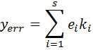
The error at each time step is given by
The above formulation accounts for the scaling factor by dividing the identity matrix by hγ. (ref: Shampine, Implementation of Rosenbrock methods). The Jacobian is assumed to be approximately equal to the partial derivative of the function with respect to the dependent variables (ref: Shampine & Reichelt, The Matlab ODE Suite). Much like the Generalized Runge Kutta methods, the Rosenbrock methods are also explicit single-step formulations that require an inversion of the A matrix at each time step. As indicated earlier, the LU-decomposition & LU-back substitution routines come in handy for these operations.
Similar to the RK methods, a variety of coefficients exist in the open literature for the 4th order Rosenbrock methods.
The Modified Rosenbrock Triple
Shampine & Reichelt (The Matlab ODE Suite) point out that the W-formulas can go “badly wrong when solving problems with solutions that exhibit very sharp changes”, especially within each time step. They propose a modified Rosenbrock Triple that advances between time steps. The Rosenbrock Triple is presented below, but re-written in a format that is scaled and conditioned.


The error estimate is given by:


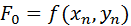
For a successful step, F2 for the completed step is the same as F0 for the next step. Shampine & Reichelt refer to it the “First Same As Last” formula, or FSAL.
The implementation of the Rosenbrock Triple is fairly straight-forward, as is obvious from the one-step formulation above. The matrix inversion in the form of LU decomposition is performed once, and the ki’s are calculated by LU back substitutions.
Wolfbrandt’s Rosenbrock method
A 2-stage Rosenbrock formulation was presented by Steihaug & Wolfbrandt (An attempt to avoid exact Jacobian and non-linear equations in the numerical solution of stiff DE’s, Mathematics of Computation, Vol. 33, No. 146, 1979, pp 521-534). In their famous paper, Shampine & Reichelt (The Matlab ODE Suite, SIAM Journal of Scientific Computing, Vol. 18, Issue 1, 1997) also introduce this “delightfully simple” 2-stage method, and refer to them as the W-formulas.
The two-step formulation is represented as follows:


The constant
 .
.
The matrix A is the same as the one defined earlier. The step-by-step process (which is similar to the generalized RK methods) can be summarized thusly:
1) Frame the matrix A
2) Create the LU-decomposed form of matrix A
3) Use LU-back substitution with f(yn) to calculate k1
4) Perform the matrix multiplication J*k1
5) Calculate k2
6) Calculate y(n+1)
As the order of the matrices increases, the computational effort for the matrix multiplication may have an impact on the computational time. Reformulation of the above method to avoid the matrix multiplication is a common technique.

Recent Comments