More on the Semi-Implicit method
The matrix formulation of the semi-implicit methods, as indicated earlier, has the advantage of avoiding an iterative procedure to converge at a solution. However, the reformulation introduces two additional complications – matrix inversion and Jacobian.
Matrix inversion can be performed by using the LU-decomposition followed by the LU-back substitution. The Jacobians can be either defined analytically or computed numerically. The analytical definitions are obviously preferred so as to avoid any numerical approximation errors with the computation, with the caveat that analytical definitions can become a little tedious to program.
Yet another generalized representation of the semi-implicit method can be stated as follows:


The above representation tends to look more like the generalized RK methods, with the obvious exception of the ‘A’ matrix and the Jacobians!
A Note on Jacobians
The matrix representation for the Backward Euler solution introduced a partial derivative term in the integration algorithm. These partial derivatives are otherwise referred to as Jacobians.
How does a partial derivative differ from its “impartial” counterpart? A partial derivative is one in which the dependent variable is differentiated with respect to only one of the other variables. Partial derivatives bring in the concept of dimensionality in a real world problem. Heat transfer problems in Mechanical Engineering are a good intuitive example.
Mathematically, let us assume a function
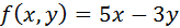
Here, y is a function of x and y. A normal derivative is usually with respect to x (assuming x is the independent variable), while the partial derivative is with respect to y. In the above case, the partial derivative, or the Jacobian of f with respect to y is

The Jacobian of a function that has multiple dependent variables is thus a matrix of partial derivatives. For example, if f is a function defined by

then the partial derivatives are

Following the above logic, the Jacobian matrix for a series of ODE’s can be represented as follows:

Matrix representation of Semi-Implicit Method
Higher order equations, or series of ODEs are more easily solved using the Semi-Implicit Method if represented as a matrix form. Thus,

Letters in bold in the above formulation are matrix representations, and I is the identity matrix. Having represented A as a matrix, the Backward Euler can now be formulated as:

The matrix formulation of the Backward Euler negates an iterative process, but introduces a matrix inversion. One matrix inversion suffices for the set of ODE’s at each time step, since the partial derivatives are constant. For a set of n ODE’s, the matrix A is of size nXn, and the variable matrix yn is nX1. A matrix multiplication thus needs to be performed to determine y(n+1).
Press et al (Press, Teukolsky, Vetterling & Flannery, Numerical Recipes, The Art of Scientific Computing) recommend LU-decompositions for the matrix inversion process, followed by the LU-back substitution. Subroutines LUDCMP and LUBKSB can be implemented for this process.
The algorithm for the semi-implicit process can be summarized as:
1) % Define step size (h), initial function y(0), initial time t0, final time tf, eps
2) nosteps = (tf – t0)/h
3) for i ← 1 to nosteps
– Calculate matrix A
– Invoke subroutine LUCDMP for A
– B ← LUDCMP (A)
– Invoke LUBKSB to compute h*B*f(yn)
– f(yn) ← LUBKSB(h*B*f(yn))
– y[i] ← y[i-1] + f(yn)
– t0 ← t0 + h
4) % Display results
Semi-Implicit Method Using Partial Derivatives
So, how does one avoid iterations and yet be able to solve the Backward Euler’s method? Press et al (Press, Teukolsky, Vetterling & Flannery, Numerical Recipes, The Art of Scientific Computing) suggest using a linearized form of the equation to represent the derivative f(yn+1). Using the principles of basic calculus,

The above representation introduces the partial derivative on the right hand side. Using this formulation and re-arranging the terms, the Backward Euler becomes:

For simple ODE’s that have just one equation, the above semi-implicit form can be easily solved by dividing the equation with the term in the square brackets, and then marching sequentially from one step to the next. The simplified formulation then becomes:


The Semi-Implicit Euler’s Method
As noted earlier, the solution of ODE’s using implicit methods (such as the Backward Euler’s method) requires an iterative procedure at each time step. Let’s take a second look at the Backward Euler’s method:

Atkinson et al (Atkinson, Han & Stewart, Numerical Solution of ODE’s) recommend a two-step approach to solving the above equation in order to avoid iterations. The two-step process can be summarized as follows:


Atkinson et al also indicate that by solving it as a two-step process, the method is no longer absolutely stable. That is, while the original Backward-Euler’s method would converge at a solution for any step size, the two-step process would not.
Methods that are used to solve for implicit formulations without an iterative process are termed as “Semi-Implicit” methods. The computational effort for iterations at each time step is avoided in the semi-implicit method, while at the same time “reasonable” stability can be guaranteed. Press et al (Press, Teukolsky, Vetterling & Flannery, Numerical Recipes, The Art of Scientific Computing) state “It is not guaranteed to be stable, but it usually is…”.
The two-body orbit problem
Orbit equations refer to a class of ODE’s in Astronomy that describes the motion of planets due to the gravitational forces that each body exerts on the others. The two-body orbit equations are represented by the following differential equations (ref: Enright & Pryce, Two Fortran Packages for Assessing Initial Value problems, ACM Transactions on Mathematical Software, Vol. 3, No. 1, pp 1-27, 1987):


The initial values are defined by

The variable step Verner’s method was employed to solve the two-body problem using an epsilon of 0.3 for the initial values. The solutions of velocity versus displacement for u and v are shown below:

The simple pendulum and its solution
The motion of an object suspended from a string that allows free swinging can be modeled using Newton’s law. The equation for a simple pendulum, which approximates the motion to a single plane, can be written as follows:

In the above equation, g is gravity, 32.2 ft/s. Given an initial angular displacement and zero initial velocity, the above equations can be solved to obtain the angular displacement and velocity of the pendulum. The 2nd order DE has to be split up into two first order ones in order to obtain a solution.
The variable-step method of Dormand & Prince was applied to solve the above IVP. The results for a 170 deg initial displacement are shown below.

A comparison of the velocity vs displacement for 45 deg and 170 deg initial values is shown below.

Variable step Fehlberg’s Method –example
Problem B2 from W.H. Enright & J.D. Pryce (Two Fortran Packages For Assessing Initial Value Methods, ACM Trans. On Mathematical Software, Vol. 13, No. 1, 1987, pp 1-27) was solved using the Variable-Step Fehlberg’s method. The equations are:


The initial conditions are 1 for all equations, with α= 3. A TOL of 1E-4 was used for the calculations, with Maxbound of 1.1 and Minbound of 0.9. The results are shown below:

The method of Verner
An example of a 7-stage method with an 8-stage error estimation was developed by Verner (Explicit Runge-Kutta Methods with Estimates of the Local Truncation Error, SIAM Journal on Numerical Analysis, Vol. 15, No. 4 (Aug., 1978), pp. 772-79). The Butcher tableau is shown below.

Once again, the generalized RK methodology can be used quite easily with the above table for the Verner’s method. The error estimate is obtained using the ycap coefficients from the last row of coefficients, and can be used to develop a variable step algorithm.
The method of Dormand & Prince
Higher order RK methods that involve 6 and higher stages of calculations at each time step are the next logical procedures. One of these methods with a 6-stage calculation, followed by a 7-stage error estimation, was developed by Dormand & Prince (Dormand & Prince, A family of embedded Runge-Kutta formulae, Journal of Computational & Applied Mathematics, Vol. 6, #1, pp 19-26). The Butcher tableau for the Dormand & Prince method is shown below.


Recent Comments