The Lotka-Volterra Predator-Prey Problem
Relationships between predators and prey are modeled using the Lotka-Volterra (LV) ODEs. The generalized form of the LV equations is:


Y1 represents the number of prey, and y2 the number of predators. Using the initial values and constants from Atkinson et al (Numerical Solution of ODEs), the Runge Kutta Merson method was used to solve the equations.

The Brusselator Problem
The Brusselator is a class of ODE’s that describe the autocatalytic reaction. The ODE’s that define the Brusselator as presented in Hairer et al (Numerical Solution of ODEs, Vol 1, Non Stiff Equations) are:

with initial values y1(0)=1.5 and y2(0)=3. The RK-Merson method with the Kaps & Rentrop variable step size algorithm was used to solve the Brusselator problem. An initial step size of 0.001 with a TOL of 0.001 was used.
The results are shown below. The first figure shows the solutions of y1 and y2 as a function of x. The power of the variable step size is evident from the “dots” in the figure. Extremely small steps are required to initiate the numerical process close to start (at t=0), while fairly generous step sizes can be used as the integration progresses along. Had a fixed step size algorithm been used for the Brusselator, the step size would have to be small all along to avoid numerical instabilities, and thus increases the computation cost significantly.
The RK-Merson Method
R.H. Merson (An operational method for the study of integration processes, Proc.
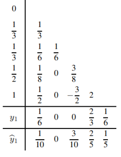
Symp. Data Processing, Weapons Research Establishment, Salisbury, Australia, 1957, pp 110-125) came up with an RK formulation of order 4. The Butcher tableau for the Merson’s method (ref: Hairer, Nørsett, Wanner, Solving ordinary differential equations, vol.1. Nonstiff problems, 2nd ed) is shown below:
Notice a second row (ycap1) at the end in the tableau. By using a 4th order formulation, followed by a 5th order estimate for the new coefficients in the last row, an error estimate can be calculated.
The generalized Butcher tableau for with error estimation then becomes
The calculations for ki’s and y(n+1) remain the same from the Generalized RK procedure. The error estimation equation is defined by
The difference between the two values of y then serves as an estimate of the error. A variable step algorithm can then be developed based on the error estimate, similar to the one presented for the Euler’s method.


Recent Comments